IGCSE · 25 September 2026 · 6 min read
IGCSE Physics half-life graphs: background correction and worked questions
Half-life questions often look like simple division by two. The difficult part is deciding what is being halved: the radioactive nuclei, the activity or the source's background-corrected count rate. A detector reading can include radiation that does not come from the source under investigation.
These original IGCSE examples show how to connect a decay curve with repeated-halving calculations. They use a fixed detector arrangement, a steady background and enough counts to reveal a useful trend. Real short measurements fluctuate, so a smooth curve represents the overall decay pattern rather than an exact prediction of each count.
Distinguish activity from measured count rate
Activity is the number of nuclear decays per second, measured in becquerels: 1 Bq means one decay per second. A detector count rate records the events detected in a given time and may be written as counts per second or counts per minute. It need not equal the activity because the detector does not necessarily register every decay from the source.
For a fixed arrangement and steady detection efficiency, the source's count rate follows its activity. Background radiation adds counts from other sources. Measure that background separately in the stated method, using comparable conditions, and subtract it. Moving the detector during the decay measurements would change how much radiation it intercepts and could imitate a change in activity.
Worked example: correct the readings before halving
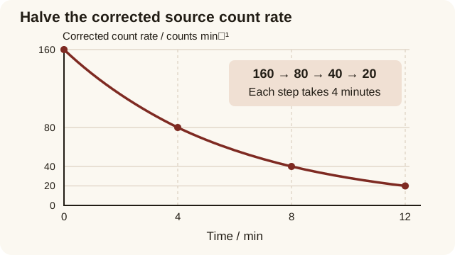
Suppose the background is 20 counts/min. A detector records total count rates of 180, 100, 60 and 40 counts/min at times 0, 4, 8 and 12 minutes. Subtract 20 from each reading to obtain source count rates of 160, 80, 40 and 20 counts/min. Each corrected value halves in 4 minutes, so the half-life is 4 minutes.
Halving the initial total of 180 to 90 counts/min would give the wrong target. A corrected source rate of 80 counts/min corresponds to a measured total of 100 counts/min because background remains present. At long times, the measured curve approaches the background level rather than zero; the corrected source curve approaches zero.
Read an interval, not just a coordinate
On a decay graph, choose a corrected count rate high enough to read clearly. Draw across to the curve, then down to the time axis. Repeat for half that count rate and subtract the two time readings. If the rate is 120 at 2.0 minutes and 60 at 6.0 minutes, the half-life is 6.0 − 2.0 = 4.0 minutes, not 6.0 minutes.
Use another pair of values to check consistency. For a single isotope under the stated model, the half-life should be similar whether you start at a higher or lower activity. A smooth best-fit curve helps represent random scatter, but it does not justify reading more decimal places than the graph scale supports. Choose widely readable levels rather than tiny values close to background.
Worked example: count how many halvings occur
A source has an initial activity of 640 Bq and a half-life of 3.0 hours. Find its activity after 12 hours. First calculate the number of half-lives: 12 / 3.0 = 4. Then halve four times: 640 → 320 → 160 → 80 → 40 Bq. The remaining fraction is 1/16, while the fraction of the original radioactive nuclei that has decayed is 15/16.
Do not subtract the same activity every three hours. The decrease gets smaller because fewer undecayed nuclei remain. After the first three hours the activity falls by 320 Bq, but over the next three hours it falls by 160 Bq. The halved fraction is constant; the numerical decrease is not.
Explain randomness without losing the predictable pattern
Radioactive decay is random: you cannot identify when a particular unstable nucleus will decay. For a large population of one isotope, however, the proportion expected to decay in a given time is predictable. This allows a reproducible half-life and a smooth overall trend even though individual detections vary between repeated measurements.
The graph does not imply that exactly half of every tiny sample must decay in each half-life. Nor does half-life mean that all nuclei disappear after two half-lives; the expected remaining fraction is then one quarter. Keep statements about the sample's statistical behaviour separate from statements about the fate of one named nucleus.
Independent practice: work backwards from a measured total
A source has half-life 5 minutes. Background is 30 counts/min, and the initial measured total is 270 counts/min. What total count rate should be expected after 15 minutes? The initial source rate is 270 − 30 = 240 counts/min. Fifteen minutes is three half-lives, so the source rate becomes 240 / 8 = 30 counts/min. Add the background back to obtain a total of 60 counts/min.
Check which answer the question requests: the source count rate would be 30, while the detector's total is 60. If you obtained 33.75, you halved the background together with the source. In revision, explain that distinction aloud, then try a new starting reading and background. A corrected calculation without the explanation can leave the original misconception intact.
Questions, explained
Choose a question for a direct answer, then explore the explanation and supporting resources. Each answer has its own link to save or share.
Why must background radiation be subtracted before finding half-life?
The background is not part of the decaying source and is approximately steady over the measurement. Halving the total detector reading therefore halves a quantity that includes a non-decaying contribution. Subtract background from each reading, find when the source contribution halves and add background back only if a later question asks for the total measured count rate.
Why does activity not become zero after two half-lives?
Each half-life halves the amount remaining, rather than removing half of the original amount again. After one half-life the expected remaining fraction is 1/2; after two it is 1/4; after three it is 1/8. The smooth model approaches zero. A real sample contains individual nuclei, whose decay times are random rather than fractions of a nucleus.
Are counts per second the same as becquerels?
Not automatically. Becquerels measure decays per second in the source, while counts per second describe what a detector records. Detection efficiency, position and background affect the reading. A background-corrected count rate can track relative activity when the arrangement stays fixed, but converting it to absolute activity needs information about what fraction of decays the detector registers.